This R models tutorial will walk users through building a Random Forest model in Azure Machine Learning and R. We will use the bike sharing dataset for this tutorial. This dataset includes the number of bikes rented for different weather conditions. From the dataset, we can build a model that will predict how many bikes will be rented during certain weather conditions.
About the Machine Learning Data
Azure Machine Learning Studio has a couple dozen built-in machine learning algorithms. But what if you need an algorithm that is not there? What if you want to customize certain algorithms? Azure can use any R or Python based machine learning package and associated algorithms! It’s called the “create model” module. With it, you can leverage the entire open-sourced R and Python communities.
The Bike Sharing dataset is a great data set for exploring Azure ML’s new R-script and R-model modules. The R-script allows for easy feature engineering from date-times and the R-model module lets us take advantage of R’s randomForest library. The data can be obtained from Kaggle; this tutorial specifically uses their “train” dataset.
The Bike Sharing dataset has 10,886 observations, each one pertaining to a specific hour from the first 19 days of each month from 2011 to 2012. The dataset consists of 11 columns that record information about bike rentals: date-time, season, working day, weather, temp, “feels like” temp, humidity, wind speed, casual rentals, registered rentals, and total rentals.
Feature Engineering & Preprocessing
There is an untapped wealth of prediction power hidden in the “datetime” column. However, it needs to be converted from its current form. Conveniently, Azure ML has a module for running R scripts, which can take advantage of R’s built-in functionality for extracting features from the date-time data.
Since Azure ML automatically converts date-time data to date-time objects, it is easiest to convert the “datetime” column to a string before sending it to the R script module. The date-time conversion function expects a string, so converting beforehand avoids formatting issues.

We now select an R-Script Module to run our feature engineering script. This module allows us to import our dataset from Azure ML, add new features, and then export our improved data set. This module has many uses beyond our use in the tutorial, which help with cleaning data and creating graphs.
Our goal is to convert the datatime column of strings into date-time objects in R, so we can take advantage of their built-in functionality. R has two internal implementations of date-times: POSIXlt and POSIXct. We found Azure ML had problems dealing with POSIXlt, so we recommend using POSIXct for any date-time feature engineering.
The function as.POSIXct converts the datetime column from a string in the specified format to a POSIXct object. Then we use the built-in functions for POSIXct objects to extract the weekday, month, and quarter for each observation. Finally, we use substr() to snip out the year and hour from the newly formatted date-time data.

Remove Problematic Data
This dataset only has one observation where weather = 4. Since this is a categorical variable, R will result in an error if it ends up in the test data split. This is because R expects the number of levels for each categorical variable to equal the number of levels found in the training data split. Therefore, it must be removed.
 #Bike sharing data set as input to the module
dataset <- maml.mapInputPort(1)

#extracting hour, weekday, month, and year from dataset
dataset$datetime <- as.POSIXct(dataset$datetime, format = "%m/%d/%Y %I:%M:%S %p")
dataset$hour  <- substr(dataset$datetime,	12,13)
dataset$weekday  <- weekdays(dataset$datetime)
dataset$month  <- months(dataset$datetime)
dataset$year  <- substr(dataset$datetime,	1,4)

#Preserving the column order
Count <- dataset[,names(dataset) %in% c("count")]
 OtherColumns <- dataset[,!names(dataset) %in% c("count")]
dataset <- cbind(OtherColumns,Count)

#Remove single observation with weather = 4 to prevent scoring model from failing
dataset <- subset(dataset, weather != '4')

#Return the dataset after appending the new features.
maml.mapOutputPort("dataset");
Define Categorical Variables
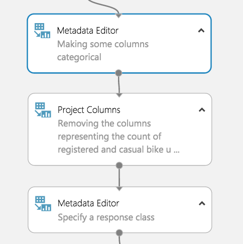
Before training our model, we must tell Azure ML which variables are categorical. To do this, we use the Metadata Editor. We used the column selector to choose the hour, weekday, month, year, season, weather, holiday, and workingday columns.
Then we select “Make categorical” under the “Categorical” dropdown.
Drop Low Value Columns
Before creating our random forest, we must identify columns that add little-to-no value for predictive modeling. These columns will be dropped.
Since we are predicting total count, the registered bike rental and casual bike rental columns must be dropped. Together, these values add up to total count, which would lead to a successful but uninformative model because the values would simply be summed to see the total count. One could train separate models to predict casual and registered bike rentals independently. Azure ML would make it very easy to include these models in our experiment after creating one for total count.

The third candidate for removal is the datetime column. Each observation has a unique date-time, so this column with just add noise to our model, especially since we extracted all the useful information (day of week, time of day etc.)
Now that the dropped columns have been chosen, drag in the “Project Columns” module to drop datetime, casual, and registered. Launch the column selector and select “All columns” from the dropdown next to “Begin With.” Change “Include” to “Exclude” using the dropdown and then select the columns we are dropping.
Specify a Response Class
We must now directly tell Azure ML which attribute we want our algorithm to train to predict by casting that attribute as a “label”.
Start by dragging in a metadata editor. Use the column selector to specify “Count” and change the “Fields” parameter to “Labels.” A dataset can only have 1 label at a time for this to work.
Our model is now ready for machine learning!

Model Building
Train Your Model
Here is where we take advantage of AzureMl’s newest feature: the Create R Model module. Now we can use R’s randomForest library and take advantage of its large number of adjustable parameters directly inside AzureML studio. Then, the model can be deployed in a web service. Previously, R models were nearly impossible to deploy to the web. For a detailed explanation of setting up data partitions and model training checkout our other tutorial here.

Similar to a native model in Azure ML, the Create R Model module connects to Train Model module. The difference is the user must provide R code for training and scoring separately. The training script goes under “Trainer R script” and takes in one dataset as an input and outputs a model. The dataset corresponds to whichever dataset gets inputted to the connected Train Module. In this case, the dataset is our training split and the model outputted is a random forest.
The scoring script goes under “Scorer R script” and has two inputs: a model and a dataset. These correspond to the model from the Train Model module and the dataset inputted to the Score Model module, which is the test split in this example. The output is a data frame of the predicted values, which get appended to the original dataset.
Make sure to appropriately label your outputs for both scripts as Azure ML expects exact variable names.
#Trainer R Script
#Input: dataset
#Output: model

library(randomForest)
model <- randomForest(Count ~ ., dataset)

 #Scorer R Script
#Input: model, dataset
#Output: scores

library(randomForest)
scores <- data.frame(predict(model, subset(dataset, select = -c(Count))))
names(scores) <- c("Predicted Count")
Evaluate Your Model

Unfortunately, AzureML’s Evaluate Model Module does not support models that use the Create R Model module, yet. We assume this feature will be added in the near future. In the meantime, we can import the results from the scored model (Score Model module) into an Execute R Script module and compute an evaluation using R. We calculated the MSE then export our result back to AzureML as a data frame.
#Results as input to module
dataset1 <- maml.mapInputPort(1)

countMSE <- mean((dataset1$Count-dataset1["Predicted Count"])^2)

evaluation <- data.frame(countMSE)
#Output evaluation
maml.mapOutputPort("evaluation");